import numpy as np
from IPython.display import Markdown
from scipy.linalg import solve_triangular

np.set_printoptions(precision=3, suppress=True)


def unit(X):
    # Scale each row to unit length.
    return X / np.linalg.norm(X, axis=1, keepdims=True)


def check(name, got, want, tolerance=1e-12):
    # Print the largest difference between two arrays and fail above the tolerance.
    error = np.abs(np.asarray(got) - np.asarray(want)).max()
    print(f"{name:<58} largest error {error:.1e}")
assert error < tolerance, nameAttention as Matrix Algebra: From Softmax to the Delta Rule
Work in progress
Attention
Linear Algebra
Work in progress. Softmax attention, linear attention, and the delta rule through matrix algebra, worked examples, and numerical checks.
This post is incomplete and will be revised. Download the notebook and figures.
Every transformer layer builds a matrix with one entry for each pair of tokens. Double the context, and the matrix grows four times. Linear attention removes the square with two moves: it changes one function, and it moves one pair of parentheses. In return it keeps a memory of fixed size, the same at the millionth token as at the first. This post explains both mechanisms as matrix algebra. Then it shows what the fixed memory forgets, and how the delta rule uses the same memory better.
The post is for readers with a degree in mathematics. It assumes you have met queries, keys and values, and it defines them again anyway. The code cells check the main identities numerically, with NumPy and SciPy.
In short
- Softmax attention is two matrix products around a row-wise softmax. Both pass through an \(n \times n\) matrix, so one head costs \(4n^2 d\) operations for \(n\) tokens.
- Softmax attention is a kernel smoother. Its kernel \(e^{q^\top k / \sqrt{d}}\) is an inner product of infinitely many features, and no finite set of features reproduces it.
- Linear attention uses a finite kernel \(\phi(q)^\top \phi(k)\) of \(r\) features. Associativity then computes an \(r \times d\) summary first, in \(4nrd\) operations.
- Under a causal mask, linear attention is a recurrent network. Its state \(S_t\) is one \(r \times d\) matrix, so generation needs the same memory at every step.
- The price is capacity. For arbitrary values, an \(r \times d\) memory returns at most \(r\) stored values free of crosstalk, and the additive rule cannot overwrite a value it has stored.
- The delta rule reads what a key already returns and writes only the difference. It is one step of gradient descent on a squared error, and each write moves the state along the key only.
- The delta rule can overwrite, and in our experiment its read error is lower than the additive rule’s at every size. It adds no capacity: no rule has a lower total squared read error than the least-squares memory, which is exact only up to \(r\) pairs.
- Training stays parallel. Inside a chunk of tokens, one triangular solve turns the values into pseudo-values, and the rest is chunked linear attention.
1. Queries, keys and values
A sequence of \(n\) tokens enters a layer as the rows of a matrix \(X \in \mathbb{R}^{n \times d_{\text{model}}}\), one vector of length \(d_{\text{model}}\) for each token. One head of attention multiplies \(X\) by three learned matrices \(W_Q, W_K, W_V \in \mathbb{R}^{d_{\text{model}} \times d}\):
\[ Q = X W_Q, \qquad K = X W_K, \qquad V = X W_V . \]
Row \(i\) of \(Q\), \(K\) and \(V\) gives three vectors of \(\mathbb{R}^d\) for token \(i\). In formulas they are column vectors.
- The query \(q_i\) describes what token \(i\) looks for.
- The key \(k_j\) describes what token \(j\) offers to a query.
- The value \(v_j\) is what token \(j\) passes on when a query selects it.
A layer runs \(h\) heads in parallel, each with \(d = d_{\text{model}} / h\). It joins their outputs side by side and multiplies them by one more learned matrix. Everything below describes one head. The values have the same length \(d\) as the keys, to keep the counts simple.
An operation is one floating-point addition or multiplication. A product of an \(a \times b\) matrix and a \(b \times c\) matrix costs \(2abc\) operations.
2. Softmax attention is two matrix products and a softmax
Definition (softmax attention). For one head, with the softmax taken over each row,
\[\operatorname{Attn}(Q, K, V) = \operatorname{softmax}\left(\frac{QK^\top}{\sqrt{d}}\right) V .\]
This is equation (1) of Vaswani et al. (2017). It is three steps.
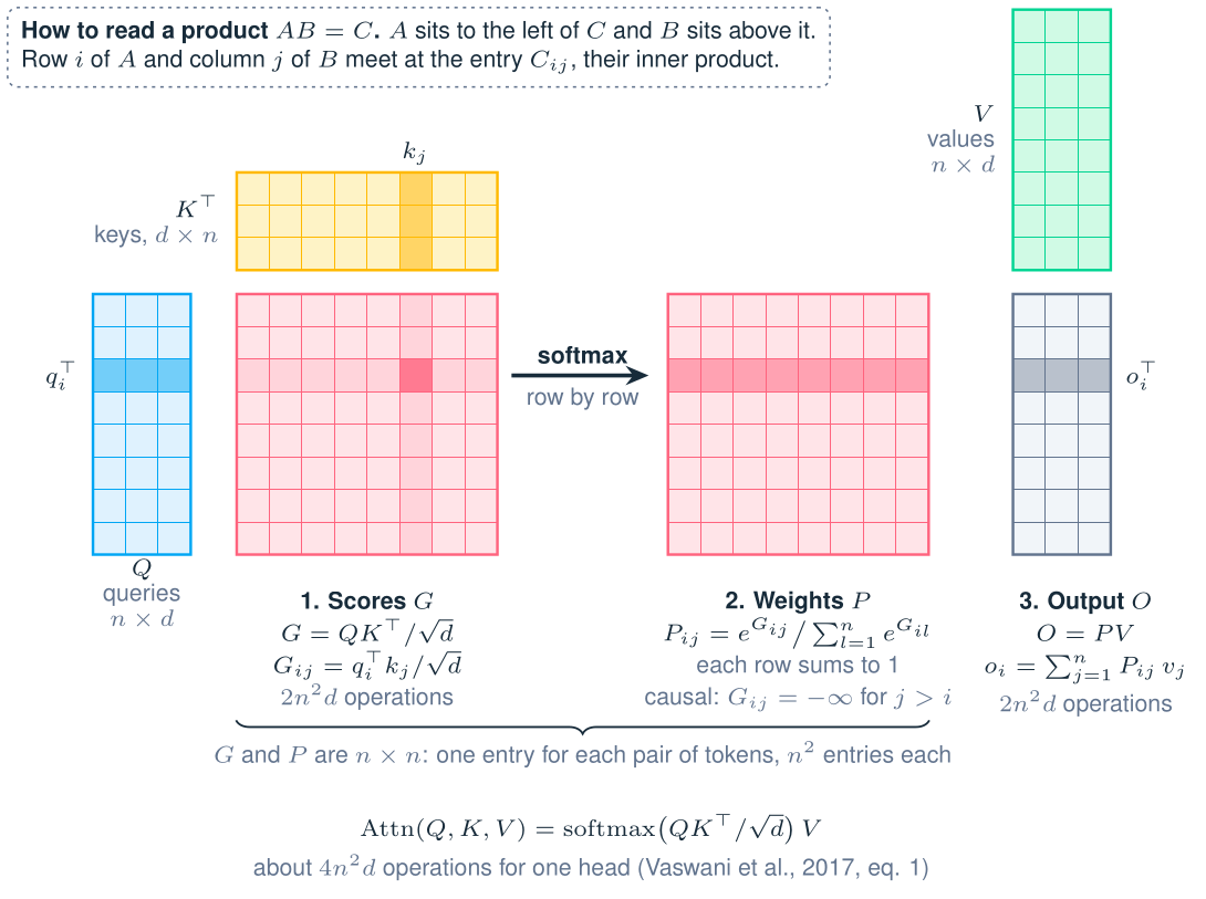
- Scores. \(G = QK^\top / \sqrt{d}\) is an \(n \times n\) matrix with entries \(G_{ij} = q_i^\top k_j / \sqrt{d}\), a scaled Gram matrix of queries against keys. It costs \(2n^2 d\) operations.
- Weights. \(P_{ij} = e^{G_{ij}} / \sum_{l=1}^{n} e^{G_{il}}\). Each row of \(P\) is a probability vector, so \(P\) is row-stochastic.
- Output. \(O = PV\), so \(o_i = \sum_{j=1}^{n} P_{ij} v_j\) is a convex combination of the values. It costs \(2n^2 d\) operations.
Figure 1. Softmax attention is two matrix products around a row-wise softmax, and both pass through an \(n \times n\) matrix.
Why divide by \(\sqrt{d}\). Suppose the entries of \(q\) and \(k\) are independent with mean 0 and variance 1. Then \(q^\top k = \sum_{m=1}^{d} q_m k_m\) has mean 0 and variance \(d\) (Vaswani et al., 2017, Section 3.2.1). Without the factor, the scores spread out as \(d\) grows. The softmax then puts almost all weight on one key, where its gradient is close to zero. The factor \(1/\sqrt{d}\) gives the scores unit variance.
The quadratic cost. The two products cost \(4n^2 d\) operations, and \(P\) has \(n^2\) entries. At \(n = 32{,}768\) tokens in 2-byte numbers, \(P\) takes 2 GiB for one head of one layer. FlashAttention computes the same output in tiles and never stores \(P\) whole (Dao et al., 2022). It removes the memory problem but keeps the \(4n^2 d\) operations.
The causal mask. A language model predicts each token from the tokens before it. So the output for token \(i\) may use only the tokens \(j \le i\). The causal mask sets \(G_{ij} = -\infty\) for \(j \gt i\) before the softmax. Then \(P\) is lower triangular, and each of its rows is still a probability vector.
Generation and the KV cache. A model generates text one token at a time. At step \(t\), the new query \(q_t\) needs every earlier key and value, \(k_1, \dots, k_t\) and \(v_1, \dots, v_t\). The model stores them instead of recomputing them. This store is the KV cache: \(2td\) numbers for each head of each layer. Step \(t\) reads the whole cache and costs about \(4td\) operations, so each step costs more than the step before.
The code subtracts each row’s largest score before it takes the exponential. The softmax does not change when a constant is added to a whole row, and the subtraction prevents overflow.
def softmax_attention(Q, K, V, causal=False):
    # O = softmax(Q K^T / sqrt(d)) V, with the row-wise softmax. Returns O and P.
    G = Q @ K.T / np.sqrt(Q.shape[1])  # the scores
    if causal:
        G = np.where(np.tril(np.ones(G.shape, dtype=bool)), G, -np.inf)
    P = np.exp(G - G.max(axis=1, keepdims=True))
    P /= P.sum(axis=1, keepdims=True)
    return P @ V, P


rng = np.random.default_rng(20261019)
Q, K, V = (rng.standard_normal((64, 8)) for _ in range(3))
_, P = softmax_attention(Q, K, V, causal=True)
check("causal softmax: each row sums to one", P.sum(axis=1), 1)
check("causal softmax: no weight above the diagonal", np.triu(P, 1), 0)
causal softmax: each row sums to one largest error 2.2e-16
causal softmax: no weight above the diagonal largest error 0.0e+003. Attention is a kernel smoother
Write the output for one token without matrices:
\[ o_i = \frac{\sum_{j=1}^{n} \kappa(q_i, k_j)\thinspace v_j}{\sum_{j=1}^{n} \kappa(q_i, k_j)}, \qquad \kappa(q, k) = e^{q^\top k / \sqrt{d}} . \]
A statistician knows this formula. It is the Nadaraya-Watson estimator: a kernel regression estimate at the point \(q_i\), from the data pairs \((k_j, v_j)\), with the kernel \(\kappa\) (Nadaraya, 1964; Tsai et al., 2019). Any nonnegative kernel gives a weighted average of the values. The choice of \(\kappa\) is the only thing that linear attention changes.
The exponential kernel is an inner product of features, but of infinitely many of them. For \(q, k \in \mathbb{R}^d\), the Taylor series gives
\[ e^{q^\top k} = \sum_{m=0}^{\infty} \frac{(q^\top k)^m}{m!} = \sum_{m=0}^{\infty} \left\langle \frac{q^{\otimes m}}{\sqrt{m!}}, \frac{k^{\otimes m}}{\sqrt{m!}} \right\rangle , \]
because \((q^\top k)^m = \langle q^{\otimes m}, k^{\otimes m} \rangle\) for the \(m\)-fold tensor power. The feature vector stacks \(q^{\otimes m} / \sqrt{m!}\) for \(m = 0, 1, 2, \dots\) and has infinitely many coordinates. If it had \(r\) coordinates, the two sums in \(o_i\) could be computed once and shared by every \(i\). Section 4 makes this precise. No finite feature map gives this kernel: the kernel matrix of Section 6.1 is nonsingular for every \(n\), and a kernel of \(r\) features gives a matrix of rank at most \(r\).
4. Linear attention: change the kernel, then reorder the product
Definition (linear attention). Choose a feature map \(\phi: \mathbb{R}^d \to [0, \infty)^r\) and use the kernel \(\kappa(q, k) = \phi(q)^\top \phi(k)\) (Katharopoulos et al., 2020):
\[o_i = \frac{\sum_{j=1}^{n} \phi(q_i)^\top \phi(k_j)\thinspace v_j}{\sum_{j=1}^{n} \phi(q_i)^\top \phi(k_j)} .\]
The scalar \(\phi(q_i)^\top \phi(k_j)\) equals \(\phi(k_j)^\top \phi(q_i)\). So the numerator is \(\sum_j v_j \phi(k_j)^\top \phi(q_i)\), and \(\phi(q_i)\) leaves both sums:
\[ o_i = \frac{M^\top \phi(q_i)}{z^\top \phi(q_i)}, \qquad M = \sum_{j=1}^{n} \phi(k_j)\thinspace v_j^\top \in \mathbb{R}^{r \times d}, \qquad z = \sum_{j=1}^{n} \phi(k_j) \in \mathbb{R}^r . \]
The matrix \(M\) and the vector \(z\) do not depend on \(i\). So they are computed once, and every output reuses them. In matrix form, this is associativity:
\[ \big( \phi(Q) \thinspace \phi(K)^\top \big) V = \phi(Q) \big( \phi(K)^\top V \big) , \]
where \(\phi(Q)\) applies \(\phi\) to each row of \(Q\). The left order builds an \(n \times n\) matrix. The right order builds the \(r \times d\) matrix \(M = \phi(K)^\top V\). Softmax attention has only the left order, because its exponential acts on each entry of \(QK^\top\), and no finite feature map reproduces it (Section 6.1).
Figure 2. The same product in two orders: an \(n \times n\) matrix first, or an \(r \times d\) matrix first.
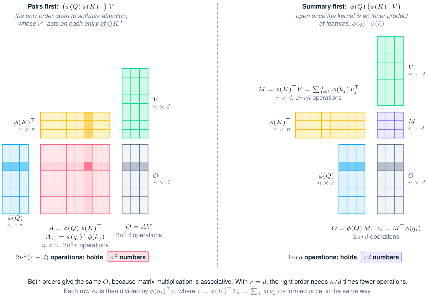
The features are nonnegative, so the weights are nonnegative. For a strictly positive map, such as the two below, the denominator is positive too, and each output is a weighted average of the values. The two maps show the range of choices.
elu + 1. Katharopoulos et al. (2020) apply \(\phi(x) = \operatorname{elu}(x) + 1\) to each coordinate, where elu is the exponential linear unit. The map gives \(x + 1\) for \(x \gt 0\) and \(e^x\) for \(x \le 0\), so \(r = d\). It is positive and cheap. It defines a new kernel and does not approximate the softmax kernel.
def elu_plus_one(X):
    # The feature map of Katharopoulos et al. (2020): elu(x) + 1, entry by entry.
    return np.where(X > 0, X + 1.0, np.exp(X))


def linear_attention_quadratic(Q, K, V, phi=elu_plus_one, causal=False):
    # Linear attention in the left order: build A = phi(Q) phi(K)^T (n x n) first.
    A = phi(Q) @ phi(K).T
    if causal:
        A = np.tril(A)
    A /= A.sum(axis=1, keepdims=True)
    return A @ V, A


def linear_attention(Q, K, V, phi=elu_plus_one):
    # Linear attention in the right order: M = phi(K)^T V (r x d) and z = phi(K)^T 1 first.
    FQ, FK = phi(Q), phi(K)
    M, z = FK.T @ V, FK.sum(axis=0)
    return (FQ @ M) / (FQ @ z)[:, None]


left, _ = linear_attention_quadratic(Q, K, V)
check("(phi(Q) phi(K)^T) V equals phi(Q) (phi(K)^T V)", left, linear_attention(Q, K, V))
(phi(Q) phi(K)^T) V equals phi(Q) (phi(K)^T V) largest error 1.0e-16Positive random features. Choromanski et al. (2021) draw \(\omega_1, \dots, \omega_r\) independently from \(N(0, I_d)\) and set
\[ \phi(x) = \frac{e^{-\lVert x \rVert^2 / 2}}{\sqrt{r}} \left( e^{\omega_1^\top x}, \dots, e^{\omega_r^\top x} \right) . \]
Then \(E_\omega[\phi(q)^\top \phi(k)] = e^{q^\top k}\) exactly, where \(E_\omega\) averages over the draws of \(\omega_1, \dots, \omega_r\). The proof is one line: \(E_\omega[e^{\omega^\top u}] = e^{\lVert u \rVert^2 / 2}\) for \(u = q + k\). To include the factor \(1/\sqrt{d}\), apply \(\phi\) to \(q / d^{1/4}\) and \(k / d^{1/4}\).
The random features give an unbiased estimate of each kernel value. The output \(o_i\), however, is a ratio of two unbiased estimates. Like the ratio estimator of survey sampling, it is consistent as \(r \to \infty\) but biased in general for a finite \(r\). The cell below checks the unbiasedness with \(r = 10^6\) features. The relative standard error of the estimate is \(\sqrt{(e^{\lVert q + k \rVert^2} - 1)/r}\), and the check allows four of them.
def positive_random_features(X, W):
    # Choromanski et al. (2021): phi(x) = exp(W x - |x|^2 / 2) / sqrt(r), W with N(0, 1) rows.
    return np.exp(X @ W.T - 0.5 * (X**2).sum(axis=1, keepdims=True)) / np.sqrt(len(W))


q, k = 0.5 * rng.standard_normal(8), 0.5 * rng.standard_normal(8)
W = rng.standard_normal((1_000_000, 8))
estimate = positive_random_features(q[None], W) @ positive_random_features(k[None], W).T
se = np.sqrt((np.exp(((q + k) ** 2).sum()) - 1) / len(W))
print(f"relative standard error of the estimate: {se:.4f}")
check("positive random features: estimate / exp(q.k)", estimate / np.exp(q @ k), 1, 4 * se)
relative standard error of the estimate: 0.0063
positive random features: estimate / exp(q.k) largest error 2.3e-03| Measure, for one head | Softmax attention | Linear attention |
|---|---|---|
| Operations | \(4n^2 d\) | \(4nrd\) |
| Largest intermediate matrix | \(n \times n\) | \(r \times d\) |
Linear attention needs fewer operations whenever \(n \gt r\). With \(r = d = 128\), that is every sequence longer than 128 tokens.
5. Under a causal mask, linear attention is a recurrent network
Under the causal mask, the sums for token \(t\) run over \(j \le t\) only:
\[ S_t = \sum_{j=1}^{t} \phi(k_j)\thinspace v_j^\top, \qquad z_t = \sum_{j=1}^{t} \phi(k_j), \qquad o_t = \frac{S_t^\top \phi(q_t)}{z_t^\top \phi(q_t)} . \]
Each sum adds one term per step, so it is a recurrence with \(S_0 = 0\) and \(z_0 = 0\):
\[ S_t = S_{t-1} + \phi(k_t)\thinspace v_t^\top, \qquad z_t = z_{t-1} + \phi(k_t) . \]
This is a recurrent network whose state is the matrix \(S_t \in \mathbb{R}^{r \times d}\), with the vector \(z_t\) beside it (Katharopoulos et al., 2020, “Transformers are RNNs”). Each step writes one rank-one matrix \(\phi(k_t) v_t^\top\) and reads the state once with \(\phi(q_t)\). A step costs about \(4rd\) operations, and the state holds \(rd + r\) numbers at every step.
Figure 3. Generation: softmax attention reads a cache that grows; linear attention reads one matrix of fixed size.
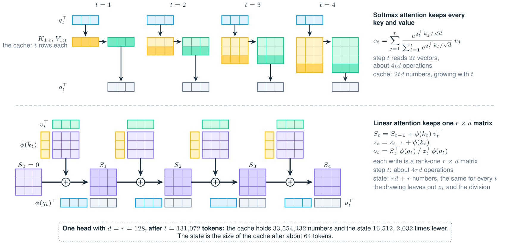
At a realistic size the difference is large. Take one head with \(d = r = 128\), after \(t = 131{,}072\) tokens. The KV cache holds 33,554,432 numbers, and the state of linear attention holds 16,512, 2,032 times fewer. The state is the size of the cache after about 64 tokens. Katharopoulos et al. (2020) report that their linear transformers were up to 4,000 times faster at autoregressive prediction of very long sequences.
def causal_linear_attention(Q, K, V, phi=elu_plus_one):
    # The recurrent form: S_t = S_{t-1} + phi(k_t) v_t^T and z_t = z_{t-1} + phi(k_t).
    FQ, FK = phi(Q), phi(K)
    S, z = np.zeros((FK.shape[1], V.shape[1])), np.zeros(FK.shape[1])
    out = np.empty((len(Q), V.shape[1]))
    for t in range(len(Q)):
        S += np.outer(FK[t], V[t])
        z += FK[t]
        out[t] = FQ[t] @ S / (FQ[t] @ z)
    return out


masked, _ = linear_attention_quadratic(Q, K, V, causal=True)
check("the recurrence equals the masked product", causal_linear_attention(Q, K, V), masked)
the recurrence equals the masked product largest error 3.3e-165.1 Training: the mask blocks the reordering
In training, the model computes all \(n\) outputs at once. The masked product is \((A \odot L) V\), where \(A = \phi(Q) \thinspace \phi(K)^\top\), \(L\) is the lower-triangular \(n \times n\) matrix of ones, and \(\odot\) multiplies entry by entry. The entry-by-entry product with \(L\) does not commute with the reordering: \((A \odot L) V \ne \phi(Q) \big( \phi(K)^\top V \big)\) in general. Row \(t\) of \((A \odot L) V\) is \(\phi(q_t)^\top S_t\), with a different \(S_t\) for each \(t\).
So there are two exact options, and neither is good alone. The loop above takes \(n\) steps in sequence, which uses matrix hardware poorly. The masked \(n \times n\) product brings back the quadratic cost. Chunks join the two. They split the sequence into blocks of \(C\) tokens, use the masked product inside each block, and carry the state between blocks. For block \(c\), with its rows \(Q_{[c]}\), \(K_{[c]}\) and \(V_{[c]}\), and its state \(S_{[c]}\) from all earlier blocks:
\[ O_{[c]} = \phi(Q_{[c]})\thinspace S_{[c]} + \big( \phi(Q_{[c]}) \thinspace \phi(K_{[c]})^\top \odot L_C \big) V_{[c]}, \qquad S_{[c+1]} = S_{[c]} + \phi(K_{[c]})^\top V_{[c]} . \]
Here \(L_C\) is the lower-triangular \(C \times C\) matrix of ones, and the normalizer follows the same pattern. The cost is about \(2nC(r + d)\) operations inside the blocks and \(4nrd\) for the states. A block of \(C = 1\) is the recurrence, and \(C = n\) is the masked quadratic product. Between them, \(C\) sets the size of the matrix products to suit the hardware. Yang et al. (2024a) build an implementation in this family that is faster than FlashAttention-2 as a single layer, even for sequences of 1K tokens.
def chunked_linear_attention(Q, K, V, C, phi=elu_plus_one):
    # Chunks of C tokens: the masked product inside a chunk, the state S across chunks.
    FQ, FK = phi(Q), phi(K)
    S, z = np.zeros((FK.shape[1], V.shape[1])), np.zeros(FK.shape[1])
    out = np.empty((len(Q), V.shape[1]))
    for c in range(0, len(Q), C):
        q, k, v = FQ[c : c + C], FK[c : c + C], V[c : c + C]
        A = np.tril(q @ k.T)  # pairs inside the chunk, under the causal mask
        out[c : c + C] = (q @ S + A @ v) / (q @ z + A.sum(axis=1))[:, None]
        S, z = S + k.T @ v, z + k.sum(axis=0)
    return out


for C in (1, 7, 16, 64):
    check(
        f"chunks of C = {C} equal the masked product", chunked_linear_attention(Q, K, V, C), masked
    )
chunks of C = 1 equal the masked product largest error 2.8e-16
chunks of C = 7 equal the masked product largest error 2.2e-16
chunks of C = 16 equal the masked product largest error 2.8e-16
chunks of C = 64 equal the masked product largest error 2.2e-166. What the fixed memory costs
The fixed memory is lossy. Three exact statements locate the loss: the rank of the attention matrix, the sharpness of its rows, and the number of values the state returns exactly.
6.1 Unmasked rank: at most \(r\) for linear attention, up to \(n\) for softmax attention
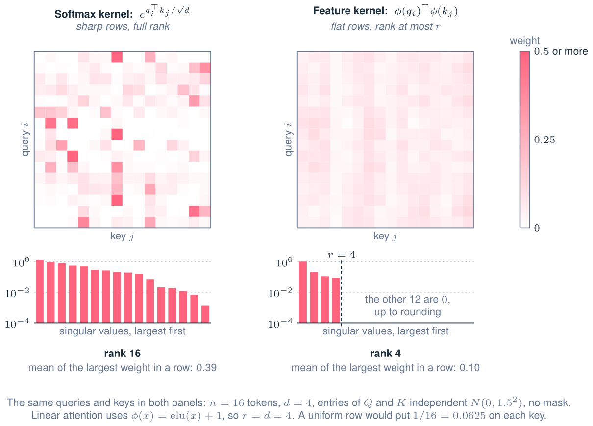
The unmasked linear attention matrix is \(D^{-1} A\), where \(A = \phi(Q) \thinspace \phi(K)^\top\) and the diagonal matrix \(D\) holds the row sums of \(A\). The matrix \(A\) is a product through \(r\) dimensions, so its rank is at most \(r\). A positive diagonal factor does not change the rank. So the unmasked linear attention matrix has rank at most \(r\), whatever \(n\) is. Causal masking can produce a full-rank matrix; this bound concerns the unmasked product.
The softmax attention matrix has no such bound, even when \(d = 1\). Let the scores be \(q_i k_j\) with distinct numbers \(q_1, \dots, q_n\) and distinct numbers \(k_1, \dots, k_n\). Then the matrix with entries \(e^{q_i k_j}\) is nonsingular, and so is \(P\).
Proof
Suppose that \(\sum_{j=1}^{n} c_j e^{q_i k_j} = 0\) for every \(i\). Then the function \(f(x) = \sum_{j=1}^{n} c_j e^{k_j x}\) has the \(n\) distinct zeros \(q_1, \dots, q_n\). We show by induction on \(m\) that an exponential sum with \(m\) distinct exponents and coefficients not all zero has at most \(m - 1\) real zeros. So \(c = 0\), and the matrix is nonsingular.
For \(m = 1\), the function \(c_1 e^{k_1 x}\) with \(c_1 \ne 0\) has no zeros. For \(m \gt 1\), the function \(g(x) = e^{-k_1 x} f(x) = c_1 + \sum_{j=2}^{m} c_j e^{(k_j - k_1) x}\) has the same zeros as \(f\). Suppose that \(g\) had at least \(m\) distinct zeros. Then by Rolle’s theorem its derivative \(g'(x) = \sum_{j=2}^{m} c_j (k_j - k_1) e^{(k_j - k_1) x}\) has at least \(m - 1\) zeros. The derivative is an exponential sum with \(m - 1\) distinct exponents. By the induction hypothesis, its coefficients \(c_j (k_j - k_1)\) are all zero, so \(c_2 = \dots = c_m = 0\). Then \(g = c_1\) is a constant with a zero, so \(c_1 = 0\) too. This contradicts the assumption that the coefficients are not all zero.
Nonsingular does not mean well conditioned. In the cell below, with six evenly spaced queries and six evenly spaced keys, the condition number of \(P\) is \(1.3 \times 10^5\). The singular values of the exponential kernel decay fast. This decay is what allows a close approximation of rank \(r\): by the Eckart-Young theorem, the smallest error in the spectral norm is the singular value number \(r + 1\).
q, k = np.linspace(-1.0, 1.0, 6), np.linspace(-0.8, 1.2, 6)
_, P1 = softmax_attention(q[:, None], k[:, None], np.eye(6))
print(
    f"d = 1, n = 6: determinant {np.linalg.det(P1):.2e}, condition number {np.linalg.cond(P1):.2e}"
)
assert np.linalg.det(P1) > 0


def attention_maps(rng, n=16, d=4, scale=1.5):
    # The softmax and the linear attention matrices of the same queries and keys.
    Q, K = scale * rng.standard_normal((n, d)), scale * rng.standard_normal((n, d))
    return softmax_attention(Q, K, np.eye(n))[1], linear_attention_quadratic(Q, K, np.eye(n))[1]


P4, A4 = attention_maps(np.random.default_rng(1))
for name, M in (("softmax", P4), ("linear", A4)):
    rank, peak = np.linalg.matrix_rank(M), M.max(axis=1).mean()
    print(f"{name:>8}: rank {rank:2d}, mean of the largest weight in a row {peak:.2f}")
d = 1, n = 6: determinant 5.09e-13, condition number 1.28e+05
softmax: rank 16, mean of the largest weight in a row 0.39
linear: rank 4, mean of the largest weight in a row 0.10Figure 4. The same queries and keys through two kernels: the softmax matrix has full rank and sharp rows; the linear one has rank \(r\) and flat rows.
6.3 Capacity: few stored values come back free of crosstalk
The state is a sum of rank-one writes, \(S_t = \sum_{j \le t} k_j v_j^\top\), with \(\phi\) folded into the keys. Reading it with the key \(k_i\) gives
\[ k_i^\top S_t = \lVert k_i \rVert^2 \thinspace v_i^\top + \sum_{j \le t, \thinspace j \ne i} (k_i^\top k_j)\thinspace v_j^\top . \]
The first term is the signal, and the second is crosstalk from the other pairs. The crosstalk vanishes for every choice of values only when \(k_i\) is orthogonal to every other stored key. For every stored pair to be read without crosstalk, the keys must be mutually orthogonal, and \(\mathbb{R}^r\) holds at most \(r\) such keys. Schlag, Irie and Schmidhuber (2021) derive this capacity limit and show that linear attention is an associative memory written by outer products.
The feature maps of Section 4 are stricter still. Both elu + 1 and positive random features have strictly positive coordinates, so \(\phi(k_i)^\top \phi(k_j) \gt 0\) for every pair of keys. No two of their keys are orthogonal. For arbitrary values, a read is then free of crosstalk only while a single pair is stored. The bound of \(r\) keys applies to feature maps with zero coordinates and to keys with mixed signs, as in the delta rule below.
Figure 5. A worked example: two orthogonal keys are stored exactly, and the third key, \((1, 1)\), adds crosstalk to every read.
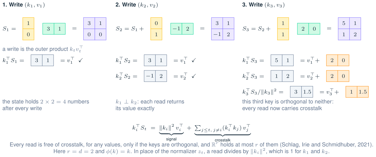
keys, values = np.array([[1, 0], [0, 1], [1, 1]]), np.array([[3, 1], [-1, 2], [2, 0]])
S2, S3 = keys[:2].T @ values[:2], keys.T @ values  # S_t = sum over j <= t of k_j v_j^T
check("Figure 5: S_2 and S_3", np.concatenate([S2, S3]), [[3, 1], [-1, 2], [5, 1], [1, 2]])
check("Figure 5: two orthogonal keys read exactly", keys[:2] @ S2, values[:2])
reads = keys @ S3 / (keys**2).sum(axis=1, keepdims=True)  # k_i^T S_3 / |k_i|^2
check("Figure 5: the crosstalk after the third write", reads - values, [[2, 0], [2, 0], [1, 1.5]])
Figure 5: S_2 and S_3 largest error 0.0e+00
Figure 5: two orthogonal keys read exactly largest error 0.0e+00
Figure 5: the crosstalk after the third write largest error 0.0e+00The trade. Linear attention replaces a memory that keeps every key and value with one \(r \times d\) matrix. Each step of generation then costs the same, at any length. But for arbitrary values the matrix returns at most \(r\) stored values free of crosstalk, and only one with a strictly positive feature map such as elu + 1. Every further pair adds crosstalk.
The evidence from trained models agrees. Arora et al. (2024) find a trade-off between the size of the state and the recall of tokens from the context. Models with a fixed state struggle at recall. Jelassi et al. (2024) prove that a two-layer transformer can copy strings of exponential length, while a model with a fixed-size state is limited by that state.
One more weakness is numerical. The denominator \(z_t^\top \phi(q_t)\) can be small. Qin et al. (2022) trace unbounded gradients in linear attention to this scaling and replace it with a normalization layer. The delta rule below has no denominator.
7. The delta rule: write only the difference
The additive rule \(S_t = S_{t-1} + k_t v_t^\top\) never removes anything. Write a new value under a key that is already stored, and the memory returns the old value and the new one added together. The delta rule fixes this with one change: before it writes, it reads what the key returns now, and it writes only the difference (Schlag, Irie and Schmidhuber, 2021). From here on, \(\phi\) is folded into the queries and keys, and the keys have unit length.
Definition (the delta rule). With a write strength \(\beta_t \in [0, 1]\),
\[u_t = \beta_t \big( v_t - S_{t-1}^\top k_t \big), \qquad S_t = S_{t-1} + k_t u_t^\top, \qquad o_t = S_t^\top q_t .\]
The vector \(S_{t-1}^\top k_t\) is the value that \(k_t\) reads before the write. The pseudo-value \(u_t\) is the correction: the new value minus the old read, scaled by \(\beta_t\). A model computes \(\beta_t\) from the token, through a sigmoid, so it learns how strongly to overwrite. Substituting \(u_t\) gives the form in the roadmap of Section 10:
\[ S_t = (I - \beta_t k_t k_t^\top)\thinspace S_{t-1} + \beta_t k_t v_t^\top . \]
Read the new state with the same key. Because \(k_t^\top k_t = 1\),
\[ S_t^\top k_t = (1 - \beta_t)\thinspace S_{t-1}^\top k_t + \beta_t v_t , \]
a convex combination of the old read and the new value. With \(\beta_t = 1\), the key returns exactly \(v_t\). Schlag et al. write the rule in this form, as the old value mixed with the new one by the write strength. DeltaNet normalizes the queries and keys to unit length, and it has no denominator (Yang et al., 2024b).
Figure 6. A new value under an old key: the additive rule keeps the old value; the delta rule reads, corrects and writes, and keeps only the new one.
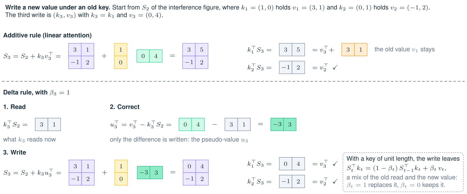
def delta_rule(Q, K, V, beta):
    # The recurrent form: read with k_t, correct by beta_t, write k_t u_t^T. Keys of unit length.
    S = np.zeros((K.shape[1], V.shape[1]))
    out = np.empty((len(Q), V.shape[1]))
    for t in range(len(Q)):
        u = beta[t] * (V[t] - K[t] @ S)  # the pseudo-value: new value minus what k_t reads now
        S += np.outer(K[t], u)
        out[t] = Q[t] @ S
    return out, S


keys, values = np.array([[1, 0], [0, 1], [1, 0]]), np.array([[3, 1], [-1, 2], [0, 4]])
_, S3 = delta_rule(keys, keys, values, np.ones(3))
check("Figure 6: additive S_3", keys.T @ values, [[3, 5], [-1, 2]])
check("Figure 6: delta-rule S_3", S3, [[0, 4], [-1, 2]])
check("Figure 6: the pseudo-value u_3", values[2] - keys[2] @ (keys[:2].T @ values[:2]), [-3, 3])
Figure 6: additive S_3 largest error 0.0e+00
Figure 6: delta-rule S_3 largest error 0.0e+00
Figure 6: the pseudo-value u_3 largest error 0.0e+007.1 One step of online regression
Think of the state as a linear map from keys to values, and score it on the newest pair with a squared error:
\[ \mathcal{L}_t(S) = \tfrac{1}{2} \lVert S^\top k_t - v_t \rVert^2, \qquad \nabla_S \mathcal{L}_t(S) = k_t \big( S^\top k_t - v_t \big)^\top . \]
One gradient step of size \(\beta_t\) from \(S_{t-1}\) is \(S_{t-1} - \beta_t k_t (S_{t-1}^\top k_t - v_t)^\top = S_{t-1} + k_t u_t^\top\): the delta rule. This is the least-mean-squares rule of Widrow and Hoff (1960), applied to the memory of a sequence model. The additive rule is a gradient step too, on the linear loss \(-\langle S^\top k_t, v_t \rangle\) (Yang et al., 2024b). The gradient of that loss is \(-k_t v_t^\top\) whatever the memory already holds, so the additive rule corrects nothing.
rng2 = np.random.default_rng(7)
S, beta = rng2.standard_normal((8, 8)), 0.7
k, v = rng2.standard_normal(8), rng2.standard_normal(8)
k /= np.linalg.norm(k)
read_correct_write = S + np.outer(k, beta * (v - k @ S))
check(
    "read-correct-write equals the Householder form",
    read_correct_write,
    (np.eye(8) - beta * np.outer(k, k)) @ S + beta * np.outer(k, v),
)
gradient = np.outer(k, S.T @ k - v)  # the gradient of |S^T k - v|^2 / 2 at S


def loss(M):
    return 0.5 * np.sum((M.T @ k - v) ** 2)


E = np.zeros_like(S)
E[2, 3] = 1e-6
check(
    "the gradient formula, against a central difference",
    (loss(S + E) - loss(S - E)) / 2e-6,
    gradient[2, 3],
    1e-8,
)
check("the delta rule is one gradient step of size beta", read_correct_write, S - beta * gradient)
check(
    "the read-back mixes the old read and the new value",
    read_correct_write.T @ k,
    (1 - beta) * (S.T @ k) + beta * v,
)
read-correct-write equals the Householder form largest error 2.2e-16
the gradient formula, against a central difference largest error 7.5e-11
the delta rule is one gradient step of size beta largest error 2.2e-16
the read-back mixes the old read and the new value largest error 3.9e-167.2 The geometry: each write moves the state along the key only
Look at one column \(s\) of the state, a vector in the key space \(\mathbb{R}^r\). The transition \(A_t = I - \beta_t k_t k_t^\top\) keeps the part of \(s\) orthogonal to \(k_t\) and multiplies the coordinate \(k_t^\top s\) by \(1 - \beta_t\). So \(A_t\) has the eigenvalue \(1 - \beta_t\) once, on \(k_t\), and the eigenvalue 1 on the orthogonal complement \(k_t^\perp\). With \(\beta_t = 1\) it is the orthogonal projection onto \(k_t^\perp\). With \(\beta_t = 2\) it is the Householder reflection. For every \(\beta_t \in [0, 2]\) and \(r \ge 2\), its spectral norm is 1, so the transition does not amplify the existing state.
The write then adds \(\beta_t v_{t,c} k_t\), where \(v_{t,c}\) is the matching coordinate of the new value. Both moves are along \(k_t\). With \(\beta_t = 1\), the write sets \(k_t^\top s = v_{t,c}\) and leaves the rest of \(s\) alone. For the linear system \(K s = V_{\cdot c}\), one equation per stored pair, this is one step of the Kaczmarz method: project the current point onto the hyperplane of one equation (Strohmer and Vershynin, 2009).
Figure 7. One write, one column: the transition moves the column along the key, and the write sets its coordinate on the key.
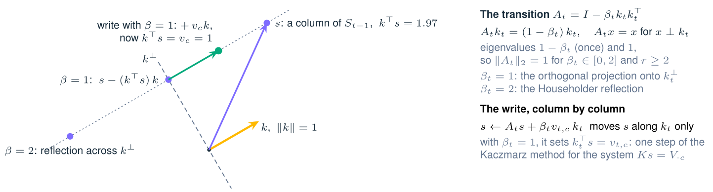
for beta in (0.0, 0.5, 1.0, 2.0):
    A_t = np.eye(8) - beta * np.outer(k, k)
    eigenvalues = np.linalg.eigvalsh(A_t)
    assert np.isclose(np.linalg.norm(A_t, 2), 1.0)
    print(
        f"beta = {beta}: eigenvalues from {eigenvalues.min():+.2f} to {eigenvalues.max():+.2f}, "
        f"spectral norm {np.linalg.norm(A_t, 2):.2f}"
    )
beta = 0.0: eigenvalues from +1.00 to +1.00, spectral norm 1.00
beta = 0.5: eigenvalues from +0.50 to +1.00, spectral norm 1.00
beta = 1.0: eigenvalues from +0.00 to +1.00, spectral norm 1.00
beta = 2.0: eigenvalues from -1.00 to +1.00, spectral norm 1.007.3 What the delta rule fixes, and what it does not
The delta rule fixes overwriting: the newest pair is always read back exactly, with \(\beta_t = 1\). It does not add capacity. An older pair is disturbed when a later key overlaps its key: a write with \(k_t\) changes the read of \(k_i\) by \((k_i^\top k_t)\thinspace u_t^\top\). No update rule can beat the capacity of the memory itself. The best \(r \times d\) memory for a set of pairs is the least-squares solution, which minimizes the total squared read error. It is exact when \(n \le r\) and the keys are linearly independent.
The cell below stores \(n\) random pairs, with keys and values drawn uniformly on the unit sphere in \(\mathbb{R}^{32}\), so \(r = d = 32\). It reads every stored key back and reports the root-mean-square read error over 200 repetitions. Theory predicts two of the columns. For the additive rule, the crosstalk of Section 6.3 has mean square \((n - 1)/r\), because \(E[(k_i^\top k_j)^2] = 1/r\) for independent random unit keys. For the least-squares memory, the residual has mean square \(\max(0, 1 - r/n)\), because the fitted values are a projection of rank \(r\).
def recall_errors(n, r=32, repetitions=200, seed=2):
    # Root-mean-square read error of three memories for n random unit pairs in R^r.
    rng = np.random.default_rng(seed)
    squared = {"additive": [], "delta, all pairs": [], "delta, 8 newest": [], "least squares": []}
    for _ in range(repetitions):
        K, V = unit(rng.standard_normal((n, r))), unit(rng.standard_normal((n, r)))
        delta = delta_rule(K, K, V, np.ones(n))[1]
        errors = {
            name: ((K @ S - V) ** 2).sum(axis=1)
            for name, S in (
                ("additive", K.T @ V),
                ("delta", delta),
                ("least squares", np.linalg.lstsq(K, V)[0]),
            )
        }
        squared["additive"].append(errors["additive"].mean())
        squared["delta, all pairs"].append(errors["delta"].mean())
        squared["delta, 8 newest"].append(errors["delta"][-8:].mean())
        squared["least squares"].append(errors["least squares"].mean())
    return {name: np.sqrt(np.mean(x)) for name, x in squared.items()}


caption = (
    "**Table 1. Root-mean-square read error of three memories with $r = d = 32$** "
    "(random unit keys and values, $\\beta_t = 1$ for the delta rule, 200 repetitions; "
    "a memory that returns zero has error 1)."
)
header = (
    "| Pairs stored $n$ | Additive | Theory | Delta, all pairs | Delta, 8 newest "
    "| Least squares | Theory |"
)
rows = [caption, "", header, "|---|---|---|---|---|---|---|"]
for n in (8, 16, 32, 64, 128):
    e = recall_errors(n)
    cells = [e["additive"], np.sqrt((n - 1) / 32), e["delta, all pairs"], e["delta, 8 newest"]]
    cells += [e["least squares"], np.sqrt(max(0, 1 - 32 / n))]
    rows.append(f"| {n} | " + " | ".join(f"{x:.3f}" for x in cells) + " |")
Markdown("\n".join(rows))
Table 1. Root-mean-square read error of three memories with \(r = d = 32\) (random unit keys and values, \(\beta_t = 1\) for the delta rule, 200 repetitions; a memory that returns zero has error 1).
| Pairs stored \(n\) | Additive | Theory | Delta, all pairs | Delta, 8 newest | Least squares | Theory |
|---|---|---|---|---|---|---|
| 8 | 0.473 | 0.468 | 0.360 | 0.360 | 0.000 | 0.000 |
| 16 | 0.681 | 0.685 | 0.537 | 0.383 | 0.000 | 0.000 |
| 32 | 0.986 | 0.984 | 0.771 | 0.414 | 0.000 | 0.000 |
| 64 | 1.403 | 1.403 | 1.030 | 0.434 | 0.707 | 0.707 |
| 128 | 1.990 | 1.992 | 1.224 | 0.447 | 0.867 | 0.866 |
The additive rule follows its theory to within 0.006 at every \(n\), and so does the least-squares memory. The delta rule lies between them. Its error is lower than the additive rule’s at every size, and its newest pairs stay readable: the 8 newest have error at most 0.45 at every \(n\). Its older pairs pay for this. From \(n = 64\) on, its error over all pairs is above 1, worse than a memory that returns zero. Below \(r\) the gap to least squares is the cost of seeing each pair once. Repeating the pairs would drive the error to zero when \(n \le r\), because the Kaczmarz method converges for a consistent system (Tanabe, 1971). The cell below checks this with 24 pairs, swept 200 times. A sequence model sees each pair only once.
rng4 = np.random.default_rng(4)
K24, V24 = unit(rng4.standard_normal((24, 32))), unit(rng4.standard_normal((24, 32)))
S = np.zeros((32, 32))
for _ in range(200):  # the same 24 pairs, written again and again with beta = 1
    for t in range(24):
        S += np.outer(K24[t], V24[t] - K24[t] @ S)
check("24 pairs swept 200 times: the reads converge", K24 @ S, V24, 1e-4)
24 pairs swept 200 times: the reads converge largest error 1.4e-058. Training the delta rule in chunks
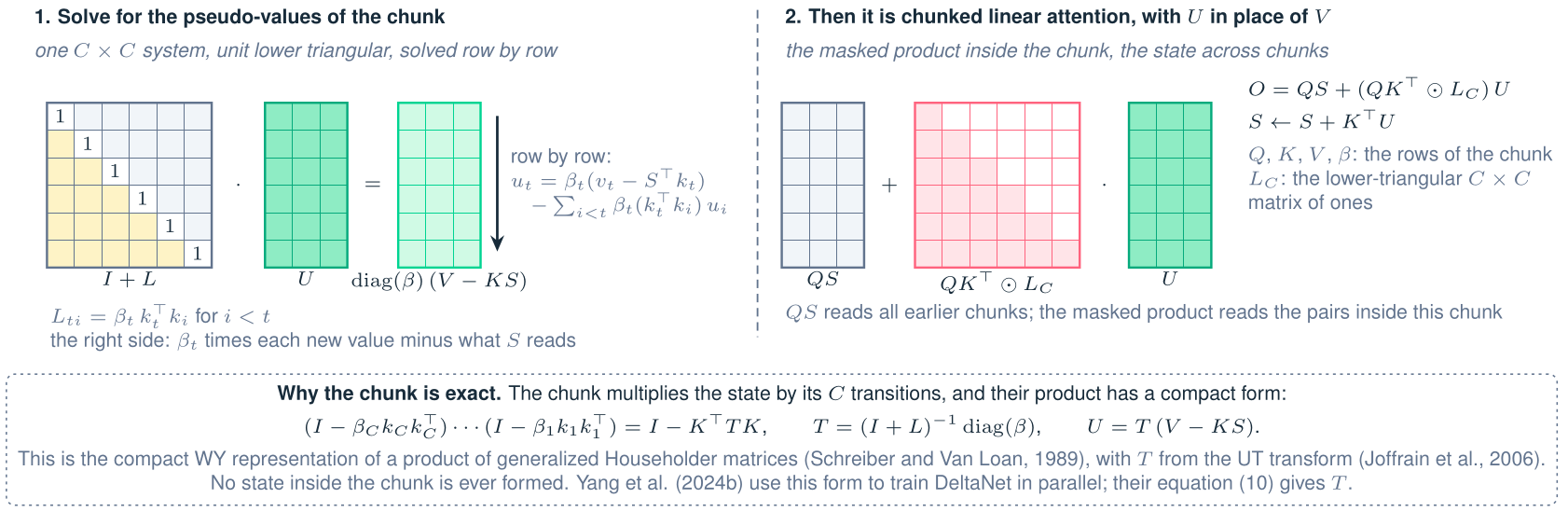
The chunks of Section 5.1 relied on the state being a plain sum of writes. The delta rule seems to break this, because each pseudo-value \(u_t\) depends on the state just before step \(t\). But the state is still a plain sum, \(S_t = S_0 + \sum_{i \le t} k_i u_i^\top\). So once the pseudo-values of a chunk are known, the chunk is ordinary chunked linear attention with \(U\) in place of \(V\) (Yang et al., 2024b, Sections 3.1 and 3.2).
The pseudo-values solve one triangular system. Inside a chunk that starts from the state \(S\), write out \(u_t = \beta_t (v_t - S_{t-1}^\top k_t)\) with \(S_{t-1} = S + \sum_{i \lt t} k_i u_i^\top\):
\[ u_t + \sum_{i \lt t} \beta_t (k_t^\top k_i)\thinspace u_i = \beta_t \big( v_t - S^\top k_t \big), \qquad \text{so} \qquad (I + L)\thinspace U = \operatorname{diag}(\beta) (V - K S) , \]
where \(L\) is strictly lower triangular with entries \(L_{ti} = \beta_t k_t^\top k_i\) for \(i \lt t\). The matrix \(I + L\) is unit lower triangular, so forward substitution solves it. Then
\[ O = Q S + (Q K^\top \odot L_C)\thinspace U, \qquad S \leftarrow S + K^\top U . \]
Substitute \(U = T (V - K S)\), with \(T = (I + L)^{-1} \operatorname{diag}(\beta)\), into the new state. It is \((I - K^\top T K) S + K^\top T V\). So the product of the chunk’s \(C\) transitions is \(I - K^\top T K\). This is the compact WY representation of a product of generalized Householder matrices (Schreiber and Van Loan, 1989), which refines the WY representation of Bischof and Van Loan (1987). The UT transform computes \(T\) (Joffrain et al., 2006). Yang et al. (2024b) use it to train DeltaNet in parallel over the sequence. Their equation (10) gives \(T\).
Figure 8. The delta rule in chunks: one triangular solve gives the pseudo-values, and the rest is chunked linear attention.
The extra work is the solve of \((I + L) U = \operatorname{diag}(\beta)(V - KS)\), the \(C \times C\) product \(KK^\top\), and the product \(KS\). Counting the masked products in full and the forward substitution at \(C^2 d\) operations, a chunk costs about \(4C^2 r + 3C^2 d + 6Crd\) operations, against \(2C^2 (r + d) + 4Crd\) for the additive rule. With \(r = d\), the delta rule costs between 1.5 and 1.75 times as much, and it is still linear in \(n\).
def chunked_delta_rule(Q, K, V, beta, C):
    # Chunks of C tokens: solve for the pseudo-values U, then chunked linear attention with U.
    S = np.zeros((K.shape[1], V.shape[1]))
    out = np.empty((len(Q), V.shape[1]))
    for c in range(0, len(Q), C):
        q, k, v, b = Q[c : c + C], K[c : c + C], V[c : c + C], beta[c : c + C]
        L = np.tril(b[:, None] * (k @ k.T), -1)  # L_ti = beta_t k_t^T k_i for i < t
        U = solve_triangular(np.eye(len(k)) + L, b[:, None] * (v - k @ S), lower=True)
        out[c : c + C] = q @ S + np.tril(q @ k.T) @ U
        S = S + k.T @ U
    return out, S


rng3 = np.random.default_rng(3)
Qd, Kd, Vd = (
    unit(rng3.standard_normal((64, 8))),
    unit(rng3.standard_normal((64, 8))),
    rng3.standard_normal((64, 8)),
)
beta = 1 / (1 + np.exp(-rng3.standard_normal(64)))  # write strengths through a sigmoid
recurrent, _ = delta_rule(Qd, Kd, Vd, beta)
for C in (1, 5, 16, 64):
    check(
        f"delta rule: chunks of C = {C} equal the recurrence",
        chunked_delta_rule(Qd, Kd, Vd, beta, C)[0],
        recurrent,
    )

C, k6, b6 = 6, Kd[:6], beta[:6]
product = np.eye(8)
for t in range(C):
    product = (np.eye(8) - b6[t] * np.outer(k6[t], k6[t])) @ product
T = solve_triangular(np.eye(C) + np.tril(b6[:, None] * (k6 @ k6.T), -1), np.diag(b6), lower=True)
check("WY form: the product of 6 transitions is I - K^T T K", product, np.eye(8) - k6.T @ T @ k6)
delta rule: chunks of C = 1 equal the recurrence largest error 4.4e-16
delta rule: chunks of C = 5 equal the recurrence largest error 8.9e-16
delta rule: chunks of C = 16 equal the recurrence largest error 8.9e-16
delta rule: chunks of C = 64 equal the recurrence largest error 1.1e-15
WY form: the product of 6 transitions is I - K^T T K largest error 2.2e-169. When each trade pays
| For one head | Softmax attention | Linear attention | Delta rule |
|---|---|---|---|
| Training operations | \(4n^2 d\) | \(2nC(r + d) + 4nrd\) in blocks of \(C\) | \(n(4Cr + 3Cd + 6rd)\) in blocks of \(C\) |
| Operations at generation step \(t\) | about \(4td\) | about \(4rd\) | about \(6rd\) |
| Memory at generation step \(t\) | \(2td\) numbers | \(rd + r\) numbers | \(rd\) numbers |
| A new value under an old key | both stay in the cache | old and new add up | the new value replaces the old (with \(\beta_t = 1\)) |
| Reading one stored pair | nearly all weight on one key, if it is a vertex of the convex hull of the keys | free of crosstalk for at most \(r\) orthogonal keys, and for one with positive features | the newest pair exactly (with \(\beta_t = 1\)); no \(r \times d\) memory holds more than \(r\) pairs exactly, for arbitrary values |
Attention is a small part of the work for short sequences. Count the operations of one layer, with an MLP of width \(4 d_{\text{model}}\). The four projections and the MLP cost \(24 n d_{\text{model}}^2\) operations. The attention products of all heads cost \(4 n^2 d_{\text{model}}\). The attention products cost more only when \(n \gt 6 d_{\text{model}}\): for \(d_{\text{model}} = 4{,}096\), beyond 24,576 tokens. Linear attention costs \(4 n r d_{\text{model}}\) for all heads. That is a fraction \(r / (6 d_{\text{model}})\) of the rest of the layer at every length: about 0.5 percent for \(r = 128\) and \(d_{\text{model}} = 4{,}096\).
Caveat (operations are not time). A GPU runs large matrix products much faster than many small ones, and time also depends on memory traffic. FlashAttention makes exact softmax attention fast in practice (Dao et al., 2022). A chunked linear attention layer can still be faster, even for sequences of 1K tokens (Yang et al., 2024a). Compare the two on the hardware that will run them.
Generation is where the fixed state pays most. Each step of softmax attention reads the whole KV cache from memory, so at long contexts the time of a step grows with the cache. Linear attention and the delta rule read about \(rd\) numbers at every step. In the example of Section 5, after 131,072 tokens, that is 2,032 times fewer numbers for linear attention and 2,048 times fewer for the delta rule.
The evidence on recall favours the delta rule. On the multi-query associative recall task, Yang et al. (2024b) report that DeltaNet performs perfectly in the hardest setting they test. Their 1.3B-parameter DeltaNet, trained on 100B tokens, outperforms Mamba and gated linear attention in perplexity and zero-shot accuracy.
10. Where this goes next
Each recurrent method in Figure 9 keeps an \(r \times d\) memory \(S_t\) and changes how step \(t\) updates it. The hybrid keeps a few full-attention layers beside them. Figure 9 shows the update rules in one notation, the notation of Kimi Team (2025).
Figure 9. The recurrent methods keep one \(r \times d\) memory and change its update; the hybrid adds back a few full-attention layers.
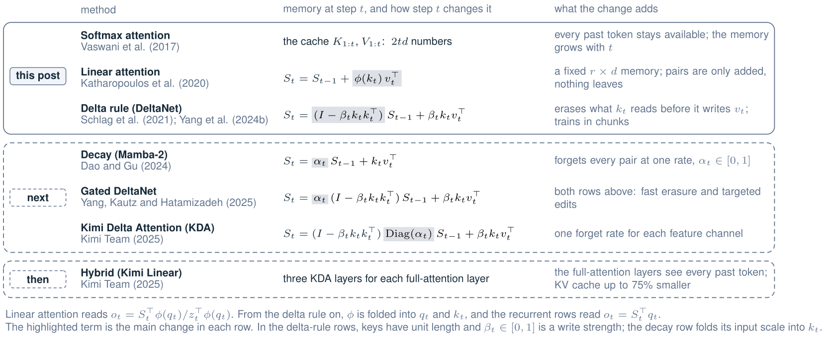
- Decay and gating. A forget rate \(\alpha_t\) shrinks old pairs. Mamba-2 uses one rate for the whole state of a head (Dao and Gu, 2024). Gated DeltaNet joins this rate to the delta rule (Yang, Kautz and Hatamizadeh, 2025). Kimi Delta Attention gives each feature channel its own rate (Kimi Team, 2025).
- Hybrids. Kimi Linear interleaves three layers of Kimi Delta Attention with one layer of full attention. The full-attention layers see every past token, and the KV cache is up to 75 percent smaller (Kimi Team, 2025).
The thread through all of them is the one this post followed. A fixed memory cannot keep everything, so each method chooses what to keep: the delta rule edits one pair at a time, decay forgets in bulk, and hybrids keep a few layers that forget nothing.
Appendix: rebuilding the figures
Each figure is a TikZ source in figures/, drawn with figures/attention-style.tex. The cell below writes the numbers that two of the figures read, then compiles every source to PDF and PNG. It needs pdflatex with TikZ and pdftocairo, and it skips the compile when they are missing. Set the PDFLATEX environment variable to choose a pdflatex.
import os
import shutil
import subprocess
import tempfile
from pathlib import Path

FIGURES = Path("figures")


def write_numbers():
    # The numbers of the attention-maps figure and of the memory comparison, as TeX macros.
    lines = [
        "% Written by attention-as-matrix-algebra.ipynb; do not edit.",
        r"\def\MapN{16}",
        r"\def\MapD{4}",
        r"\def\MapScale{1.5}",
        rf"\def\MapUniform{{{1 / 16:.4f}}}",
    ]
    for name, M in (("Softmax", P4), ("Linear", A4)):
        sv = np.linalg.svd(M, compute_uv=False)
        nonzero = sv[sv > 1e-12]  # the rest are zero up to rounding, below 1e-15
        weights = ", ".join(f"{i}/{j}/{M[i, j]:.4f}" for i in range(16) for j in range(16))
        logs = ", ".join(f"{i}/{np.log10(s):.3f}" for i, s in enumerate(nonzero))
        lines += [
            rf"\def\{name}Weights{{{weights}}}",
            rf"\def\{name}LogSingular{{{logs}}}",
            rf"\def\{name}Zeros{{{len(sv) - len(nonzero)}}}",
            rf"\def\{name}Rank{{{np.linalg.matrix_rank(M)}}}",
            rf"\def\{name}MaxWeight{{{M.max(axis=1).mean():.2f}}}",
        ]
    (FIGURES / "attention-maps-numbers.tex").write_text("\n".join(lines) + "\n")
    d, t = 128, 131_072  # one head with d = r = 128, after t tokens
    cache, state = 2 * t * d, d * d + d
    (FIGURES / "memory-numbers.tex").write_text(
        "\n".join(
            [
                "% Written by attention-as-matrix-algebra.ipynb; do not edit.",
                rf"\def\HeadDim{{{d}}}",
                rf"\def\Tokens{{{group(t)}}}",
                rf"\def\CacheNumbers{{{group(cache)}}}",
                rf"\def\StateNumbers{{{group(state)}}}",
                rf"\def\CacheRatio{{{group(round(cache / state))}}}",
                rf"\def\BreakEven{{{state // (2 * d)}}}",
            ]
        )
        + "\n"
    )
    print(
        f"cache {cache:,} numbers, state {state:,}, ratio {cache / state:.0f}; P at n = 32,768: "
        f"{32_768**2 * 2 / 2**30:g} GiB"
    )


def group(x):
    # Thousands separators that TeX math keeps tight: 131{,}072.
    return f"{x:,}".replace(",", "{,}")


def render(tex):
    # Compile one standalone TikZ source to PDF, then to a PNG at 220 dots per inch.
    pdflatex = os.environ.get("PDFLATEX", "pdflatex")
    with tempfile.TemporaryDirectory() as tmp:
        subprocess.run(
            [
                pdflatex,
                "-interaction=nonstopmode",
                "-halt-on-error",
                f"-output-directory={tmp}",
                tex.name,
            ],
            cwd=tex.parent,
            check=True,
            capture_output=True,
        )
        shutil.copyfile(Path(tmp) / tex.with_suffix(".pdf").name, tex.with_suffix(".pdf"))
    subprocess.run(
        [
            "pdftocairo",
            "-png",
            "-r",
            "220",
            "-singlefile",
            tex.with_suffix(".pdf"),
            tex.with_suffix(""),
        ],
        check=True,
    )


write_numbers()
sources = sorted(
    p
    for p in FIGURES.glob("*.tex")
    if p.stem not in ("attention-style",) and not p.stem.endswith("-numbers")
)
if shutil.which(os.environ.get("PDFLATEX", "pdflatex")) and shutil.which("pdftocairo"):
    for tex in sources:
        render(tex)
    print("compiled:", ", ".join(p.stem for p in sources))
else:
    print("pdflatex or pdftocairo not found; the figures were not recompiled")
cache 33,554,432 numbers, state 16,512, ratio 2032; P at n = 32,768: 2 GiB
compiled: attention-maps, cache-and-state, chunked-delta, householder, interference, overwrite, reordering, series-roadmap, softmax-attention-productsReferences
- Arora, S., Eyuboglu, S., Zhang, M., et al. (2024). Simple linear attention language models balance the recall-throughput tradeoff. International Conference on Machine Learning (ICML) 2024. arXiv:2402.18668
- Bischof, C. and Van Loan, C. (1987). The WY representation for products of Householder matrices. SIAM Journal on Scientific and Statistical Computing 8(1), s2–s13. doi:10.1137/0908009
- Choromanski, K., Likhosherstov, V., Dohan, D., et al. (2021). Rethinking attention with Performers. International Conference on Learning Representations (ICLR) 2021. arXiv:2009.14794
- Dao, T., Fu, D. Y., Ermon, S., Rudra, A. and Ré, C. (2022). FlashAttention: Fast and memory-efficient exact attention with IO-awareness. Advances in Neural Information Processing Systems (NeurIPS) 2022. arXiv:2205.14135
- Dao, T. and Gu, A. (2024). Transformers are SSMs: Generalized models and efficient algorithms through structured state space duality. ICML 2024. arXiv:2405.21060
- Jelassi, S., Brandfonbrener, D., Kakade, S. M. and Malach, E. (2024). Repeat after me: Transformers are better than state space models at copying. ICML 2024. arXiv:2402.01032
- Joffrain, T., Low, T. M., Quintana-Ortí, E. S., van de Geijn, R. and Van Zee, F. G. (2006). Accumulating Householder transformations, revisited. ACM Transactions on Mathematical Software 32(2), 169–179. doi:10.1145/1141885.1141886
- Katharopoulos, A., Vyas, A., Pappas, N. and Fleuret, F. (2020). Transformers are RNNs: Fast autoregressive transformers with linear attention. ICML 2020. arXiv:2006.16236
- Kimi Team (2025). Kimi Linear: An expressive, efficient attention architecture. Preprint. arXiv:2510.26692
- Nadaraya, E. A. (1964). On estimating regression. Theory of Probability and Its Applications 9(1), 141–142. doi:10.1137/1109020
- Qin, Z., Han, X., Sun, W., Li, D., Kong, L., Barnes, N. and Zhong, Y. (2022). The devil in linear transformer. Conference on Empirical Methods in Natural Language Processing (EMNLP) 2022. arXiv:2210.10340
- Schlag, I., Irie, K. and Schmidhuber, J. (2021). Linear transformers are secretly fast weight programmers. ICML 2021. arXiv:2102.11174
- Schreiber, R. and Van Loan, C. (1989). A storage-efficient WY representation for products of Householder transformations. SIAM Journal on Scientific and Statistical Computing 10(1), 53–57. doi:10.1137/0910005
- Strohmer, T. and Vershynin, R. (2009). A randomized Kaczmarz algorithm with exponential convergence. Journal of Fourier Analysis and Applications 15(2), 262–278. doi:10.1007/s00041-008-9030-4
- Tanabe, K. (1971). Projection method for solving a singular system of linear equations and its applications. Numerische Mathematik 17(3), 203–214. doi:10.1007/BF01436376
- Tsai, Y.-H. H., Bai, S., Yamada, M., Morency, L.-P. and Salakhutdinov, R. (2019). Transformer dissection: A unified understanding of Transformer’s attention via the lens of kernel. EMNLP-IJCNLP 2019. arXiv:1908.11775
- Vaswani, A., Shazeer, N., Parmar, N., Uszkoreit, J., Jones, L., Gomez, A. N., Kaiser, Ł. and Polosukhin, I. (2017). Attention is all you need. NeurIPS 2017. arXiv:1706.03762
- Widrow, B. and Hoff, M. E. (1960). Adaptive switching circuits. IRE WESCON Convention Record, Part 4, 96–104. PDF at Stanford
- Yang, S., Wang, B., Shen, Y., Panda, R. and Kim, Y. (2024a). Gated linear attention transformers with hardware-efficient training. ICML 2024. arXiv:2312.06635
- Yang, S., Wang, B., Zhang, Y., Shen, Y. and Kim, Y. (2024b). Parallelizing linear transformers with the delta rule over sequence length. NeurIPS 2024. arXiv:2406.06484
- Yang, S., Kautz, J. and Hatamizadeh, A. (2025). Gated delta networks: Improving Mamba2 with delta rule. ICLR 2025. arXiv:2412.06464